Osculating circle

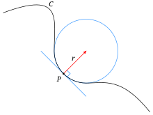
 In differential geometry of curves, the osculating circle of a sufficiently smooth plane curve at a given point p on the curve has been traditionally defined as the circle passing through p and a pair of additional points on the curve infinitesimally close to p. Its center lies on the inner normal line, and its curvature defines the curvature of the given curve at that point. This circle, which is the one among all tangent circles at the given point that approaches the curve most tightly, was named circulus osculans (Latin for "kissing circle") by Leibniz.

An osculating circle

Osculating circles of the Archimedean spiral, nested by the Tait–Kneser theorem. "The spiral itself is not drawn: we see it as the locus of points where the circles are especially close to each other."^[1]

The center and radius of the osculating circle at a given point are called center of curvature and radius of curvature of the curve at that point. A geometric construction was described by Isaac Newton in his Principia:

There being given, in any places, the velocity with which a body describes a given figure, by means of forces directed to some common centre: to find that centre.

— Isaac Newton, Principia; PROPOSITION V. PROBLEM I.

Nontechnical descriptionEdit

Imagine a car moving along a curved road on a vast flat plane. Suddenly, at one point along the road, the steering wheel locks in its present position. Thereafter, the car moves in a circle that "kisses" the road at the point of locking. The curvature of the circle is equal to that of the road at that point. That circle is the osculating circle of the road curve at that point.

Mathematical descriptionEdit

See also: Curvature

Let γ(s) be a regular parametric plane curve, where s is the arc length (the natural parameter). This determines the unit tangent vector T(s), the unit normal vector N(s), the signed curvature k(s) and the radius of curvature R(s) at each point for which s is composed:

$$

Suppose that P is a point on γ where k ≠ 0. The corresponding center of curvature is the point Q at distance R along N, in the same direction if k is positive and in the opposite direction if k is negative. The circle with center at Q and with radius R is called the osculating circle to the curve γ at the point P.

If C is a regular space curve then the osculating circle is defined in a similar way, using the principal normal vector N. It lies in the osculating plane, the plane spanned by the tangent and principal normal vectors T and N at the point P.

The plane curve can also be given in a different regular parametrization

${\displaystyle \gamma (t)={\begin{bmatrix}x_{1}(t)\\x_{2}(t)\end{bmatrix}}}$

where regular means that ${\displaystyle \gamma '(t)\neq 0}$ for all ${\displaystyle t}$. Then the formulas for the signed curvature k(t), the normal unit vector N(t), the radius of curvature R(t), and the center Q(t) of the osculating circle are

${\displaystyle k(t)={\frac {x_{1}'(t)\cdot x_{2}''(t)-x_{1}''(t)\cdot x_{2}'(t)}{\left(x_{1}'\left(t\right)^{2}+x_{2}'\left(t\right)^{2}\right)^{\frac {3}{2}}}},\qquad N(t)={\frac {1}{\|\gamma '(t)\|}}\cdot {\begin{bmatrix}-x_{2}'(t)\\x_{1}'(t)\end{bmatrix}}}$

${\displaystyle R(t)=\left|{\frac {\left(x_{1}'\left(t\right)^{2}+x_{2}'\left(t\right)^{2}\right)^{\frac {3}{2}}}{x_{1}'(t)\cdot x_{2}''(t)-x_{1}''(t)\cdot x_{2}'(t)}}\right|\qquad {\text{and}}\qquad Q(t)=\gamma (t)+{\frac {1}{k(t)\cdot \|\gamma '(t)\|}}\cdot {\begin{bmatrix}-x_{2}'(t)\\x_{1}'(t)\end{bmatrix}}\,.}$

Cartesian coordinatesEdit

We can obtain the center of the osculating circle in Cartesian coordinates if we substitute t = x and y = f(x) for some function f. If we do the calculations the results for the X and Y coordinates of the center of the osculating circle are:

${\displaystyle x_{c}=x-f'{\frac {1+f'^{2}}{f''}}\quad {\text{and}}\quad y_{c}=f+{\frac {1+f'^{2}}{f''}}}$

Direct geometrical derivationEdit

Consider three points ${\textstyle P_{0}}$,${\textstyle P_{1}}$ and ${\textstyle P_{2}}$, where ${\textstyle P_{i}=(x_{i},y_{i})}$. To find the center of the circle that passes through these points, we have first to find the segment bisectors of ${\textstyle P_{0}P_{1}}$ and ${\textstyle P_{1}P_{2}}$ and then the point ${\textstyle C}$ where these lines cross. Therefore, the coordinates of ${\textstyle C}$ are obtained through solving a linear system of two equations:

$${\displaystyle \left(\delta x_{i}\right)x_{c}+\left(\delta y_{i}\right)y_{c}={\frac {1}{2}}\left(\delta ^{2}x_{i}+\delta ^{2}y_{i}\right)\,\,\,\,i=1,2}$$

where ${\textstyle \delta u_{i}=u_{i}-u_{i-1}}$, ${\textstyle \delta ^{2}u_{i}=u_{i}^{2}-u_{i-1}^{2}}$ for ${\textstyle u=x,y}$.

Consider now the curve ${\textstyle P=P(\tau )}$ and set ${\textstyle P_{0}=P(\tau -d\tau )}$, ${\textstyle P_{1}=P(\tau )}$ and ${\textstyle P_{2}=P(\tau +d\tau )}$. To the second order in ${\textstyle d\tau }$, we have

$${\displaystyle {\begin{aligned}\delta u_{1}=&{\dot {u}}d\tau -{\frac {1}{2}}{\ddot {u}}d\tau ^{2}\\\delta ^{2}u_{1}=&2u{\dot {u}}d\tau -d\tau ^{2}\left({\dot {u}}^{2}+u{\ddot {u}}\right)\end{aligned}}}$$

and a similar expression for ${\textstyle \delta u_{2}}$ and ${\textstyle \delta ^{2}u_{2}}$ where the sign of ${\textstyle d\tau ^{2}}$ is reversed. Developing the equation for ${\textstyle x_{c},y_{c}}$ and grouping the terms in ${\textstyle d\tau }$ and ${\textstyle d\tau ^{2}}$, we obtain

$${\displaystyle {\begin{aligned}{\dot {x}}(x_{c}-x)+{\dot {y}}(y_{c}-y)=&0\\{\ddot {x}}(x_{c}-x)+{\ddot {y}}(y_{c}-y)=&{\dot {x}}^{2}+{\dot {y}}^{2}\end{aligned}}}$$

Denoting ${\textstyle \mathbf {r} ={\overrightarrow {P_{1}C}}}$, the first equation means that ${\textstyle \mathbf {r} }$ is orthogonal to the unit tangent vector at ${\textstyle P_{1}}$ :

$${\displaystyle \mathbf {r} .\mathbf {t} =0}$$

The second relation means that

$${\displaystyle \mathbf {k} .\mathbf {r} =1}$$

where

$${\displaystyle \mathbf {k} ={\frac {d\mathbf {t} }{ds}}=({\ddot {x}},{\ddot {y}})/\left({\dot {x}}^{2}+{\dot {y}}^{2}\right)}$$

is the curvature vector. In plane geometry, ${\textstyle \mathbf {k} }$ is orthogonal to ${\textstyle \mathbf {t} }$ because

$${\displaystyle \mathbf {t} .\mathbf {k} =\mathbf {t} {\frac {d\mathbf {t} }{ds}}={\frac {1}{2}}{\frac {d(\mathbf {t} .\mathbf {t} )}{ds}}={\frac {1}{2}}{\frac {d(1)}{ds}}=0}$$

Therefore ${\textstyle \mathbf {k} .\mathbf {r} =k.r}$ and the radius of the osculating circle is precisely the inverse of the curvature.

Solving the equation for the coordinates of ${\textstyle C}$, we find

$${\displaystyle {\begin{aligned}x_{c}-x=&{\frac {{\dot {y}}\left({\dot {x}}^{2}+{\dot {y}}^{2}\right)}{{\dot {y}}{\ddot {x}}-{\dot {x}}{\ddot {y}}}}\\y_{c}-y=&{\frac {-{\dot {x}}\left({\dot {x}}^{2}+{\dot {y}}^{2}\right)}{{\dot {y}}{\ddot {x}}-{\dot {x}}{\ddot {y}}}}\end{aligned}}}$$

Osculating circle as a minimization problemEdit

Consider a curve ${\textstyle C}$ defined intrinsically by the equation

$${\displaystyle f(x,y)=0}$$

which we can envision as the section of the surface ${\textstyle z=f(x,y)}$ by the plane ${\textstyle z=0}$. The normal ${\textstyle \mathbf {n} }$ to the curve at a point ${\textstyle P_{0}=(x_{0},y_{0})}$ is the gradient at this point

$${\displaystyle \mathbf {n} =(f_{x},f_{y})}$$

Therefore, the centers of the tangent circles ${\textstyle B_{\alpha }}$ are given by

${\displaystyle X_{c}=x_{0}-\alpha f_{x}\,\,;\,\,Y_{c}=y_{0}-\alpha f_{y}}$

where ${\textstyle \alpha }$ is parameter. For a given ${\textstyle \alpha ,}$the radius ${\textstyle R}$ of ${\textstyle B_{\alpha }}$ is

$${\displaystyle R^{2}=\alpha ^{2}(f_{x}^{2}+f_{y}^{2})}$$

We wish to find, among all possible circles ${\textstyle B_{\alpha }}$, the one that matches best the curve.

The coordinates of a point ${\textstyle P_{1}\in B_{\alpha }}$ can be written as

$${\displaystyle x_{1}=X_{c}+R\cos \theta \,\,;\,\,y_{1}=Y_{c}+R\sin \theta }$$

where for ${\textstyle \theta =\theta _{0}}$, ${\textstyle P_{1}=P_{0}}$, i.e.

$${\displaystyle R\cos \theta _{0}=\alpha f_{x}\,\,;\,\,R\sin \theta _{0}=\alpha f_{y}}$$

Consider now a point ${\textstyle P_{1}\in B_{\alpha }}$ close to ${\textstyle P_{0}}$, where its “angle” is ${\textstyle \theta _{1}=\theta _{0}+d\theta }$. Developing the trigonometric functions to the second order in ${\textstyle d\theta }$ and using the above relations, coordinates of ${\displaystyle P_{1}}$ are

$${\displaystyle {\begin{aligned}x_{1}=&x_{0}-\alpha f_{y}d\theta -{\frac {1}{2}}\alpha f_{x}\left(d\theta \right)^{2}\\y_{1}=&y_{0}+\alpha f_{x}d\theta -{\frac {1}{2}}\alpha f_{y}\left(d\theta \right)^{2}\end{aligned}}}$$

We can now evaluate the function ${\textstyle f(,)}$ at the point ${\textstyle P_{1}}$ and its variation ${\displaystyle f(x_{1},y_{1})-f(x_{0},y_{0})}$. The variation is zero to the first order in ${\textstyle d\theta }$ by construction (to the first order in ${\textstyle \theta }$, ${\textstyle P_{1}}$ is on the tangent line to the curve ${\textstyle C}$). The variation proportional to ${\displaystyle (d\theta )^{2}}$ is

$${\displaystyle df=-{\frac {1}{2}}\alpha \left(f_{x}^{2}+f_{y}^{2}\right)+{\frac {1}{2}}\alpha ^{2}\left(f_{y}^{2}f_{xx}+f_{x}^{2}f_{yy}-f_{x}f_{y}f_{xy}\right)}$$

and this variation is zero if we choose

$${\displaystyle \alpha =\left(f_{x}^{2}+f_{y}^{2}\right){\bigg /}\left(f_{y}^{2}f_{xx}+f_{x}^{2}f_{yy}-f_{x}f_{y}f_{xy}\right)}$$

Therefore the radius of the osculating circle is

$${\displaystyle R=\left|{\frac {\left(f_{x}^{2}+f_{y}^{2}\right)^{3/2}}{\left(f_{y}^{2}f_{xx}+f_{x}^{2}f_{yy}-f_{x}f_{y}f_{xy}\right)}}\right|}$$

For an explicit function ${\displaystyle f(x,y)=y-g(x)}$, we find the results of the preceding section.

PropertiesEdit

For a curve C given by a sufficiently smooth parametric equations (twice continuously differentiable), the osculating circle may be obtained by a limiting procedure: it is the limit of the circles passing through three distinct points on C as these points approach P.^[2] This is entirely analogous to the construction of the tangent to a curve as a limit of the secant lines through pairs of distinct points on C approaching P.

The osculating circle S to a plane curve C at a regular point P can be characterized by the following properties:

• The circle S passes through P.
• The circle S and the curve C have the common tangent line at P, and therefore the common normal line.
• Close to P, the distance between the points of the curve C and the circle S in the normal direction decays as the cube or a higher power of the distance to P in the tangential direction.

This is usually expressed as "the curve and its osculating circle have the second or higher order contact" at P. Loosely speaking, the vector functions representing C and S agree together with their first and second derivatives at P.

If the derivative of the curvature with respect to s is nonzero at P then the osculating circle crosses the curve C at P. Points P at which the derivative of the curvature is zero are called vertices. If P is a vertex then C and its osculating circle have contact of order at least three. If, moreover, the curvature has a non-zero local maximum or minimum at P then the osculating circle touches the curve C at P but does not cross it.

The curve C may be obtained as the envelope of the one-parameter family of its osculating circles. Their centers, i.e. the centers of curvature, form another curve, called the evolute of C. Vertices of C correspond to singular points on its evolute.

Within any arc of a curve C within which the curvature is monotonic (that is, away from any vertex of the curve), the osculating circles are all disjoint and nested within each other. This result is known as the Tait-Kneser theorem.^[1]

ExamplesEdit

ParabolaEdit

The osculating circle of the parabola at its vertex has radius 0.5 and fourth order contact.

For the parabola

${\displaystyle \gamma (t)={\begin{bmatrix}t\\t^{2}\end{bmatrix}}}$

the radius of curvature is

${\displaystyle R(t)=\left|{\frac {\left(1+4\cdot t^{2}\right)^{\frac {3}{2}}}{2}}\right|}$

At the vertex ${\displaystyle \gamma (0)={\begin{bmatrix}0\\0\end{bmatrix}}}$ the radius of curvature equals R(0) = 0.5 (see figure). The parabola has fourth order contact with its osculating circle there. For large t the radius of curvature increases ~ t³, that is, the curve straightens more and more.

Lissajous curveEdit

A Lissajous curve with ratio of frequencies (3:2) can be parametrized as follows

${\displaystyle \gamma (t)={\begin{bmatrix}\cos(3t)\\\sin(2t)\end{bmatrix}}.}$

It has signed curvature k(t), normal unit vector N(t) and radius of curvature R(t) given by

${\displaystyle k(t)={\frac {6\cos(t)(8(\cos t)^{4}-10(\cos t)^{2}+5)}{(232(\cos t)^{4}-97(\cos t)^{2}+13-144(\cos t)^{6})^{3/2}}}\,,}$

${\displaystyle N(t)={\frac {1}{\|\gamma '(t)\|}}\cdot {\begin{bmatrix}-2\cos(2t)\\-3\sin(3t)\end{bmatrix}}}$

and

${\displaystyle R(t)=\left|{\frac {\left(232\cos ^{4}(t)-97\cos ^{2}(t)+13-144\cos ^{6}(t)\right)^{3/2}}{6\cos(t)\left(8\cos ^{4}(t)-10\cos ^{2}(t)+5\right)}}\right|.}$

See the figure for an animation. There the "acceleration vector" is the second derivative ${\textstyle {\frac {\mathrm {d} ^{2}\gamma (s)}{\mathrm {d} s^{2}}}}$ with respect to the arc length s.

CycloidEdit

Cycloid (blue), its osculating circle (red) and evolute (green).

A cycloid with radius r can be parametrized as follows:

${\displaystyle \gamma (t)={\begin{bmatrix}r\left(t-\sin t\right)\\r\left(1-\cos t\right)\end{bmatrix}}}$

Its curvature is given by the following formula:^[3]

${\displaystyle \kappa (t)=-{\frac {\left|\csc \left({\frac {t}{2}}\right)\right|}{4r}}}$

which gives:

${\displaystyle R(t)={\frac {4r}{\left|\csc \left({\frac {t}{2}}\right)\right|}}}$

This article uses material from the Wikipedia article  Metasyntactic variable, which is released under the  Creative Commons Attribution-ShareAlike 3.0 Unported License.